Encoding, Decoding, and Learning: The Math of Sequence-to-Sequence Translation

In this post, you’ll explore the mathematical foundations of sequence-to-sequence (seq2seq) models for machine translation. We’ll focus on the RNN Encoder–Decoder architecture, which consists of two main components: an encoder RNN and a decoder RNN. As an example, we’ll see how this model can be trained to translate English phrases into French 🇬🇧➡️🇫🇷.

Definition¶

$\textcolor{green}{\text{Sequence-to-Sequence (Seq2Seq) Translation }}$¶

Sequence-to-Sequence (Seq2Seq) is a deep learning framework designed to convert an input sequence (e.g., a sentence in French) into an output sequence (e.g., its English translation). It consists of two main components:

• $\textcolor{green}{\text{ Encoder}}$ – Processes the input sequence and compresses it into a $\textcolor{green}{\text{context vector}}$, a fixed-length representation capturing the input’s semantics.

• $\textcolor{green}{\text{ Decoder}}$ – Generates the output sequence $\textcolor{green}{\text{step-by-step}}$, conditioned on the context vector from the encoder.

Key Features

• Handles variable-length input and output sequences (e.g., translating sentences of different lengths).
• Supports various architectures: RNNs, LSTMs, GRUs, and more recently, Transformers (state-of-the-art).
• Trained end-to-end using teacher forcing i.e., during training, the decoder is fed the true previous token rather than its own prediction.

$\textcolor{green}{\text{ }}$

Preliminaries: Recurrent Neural Networks¶

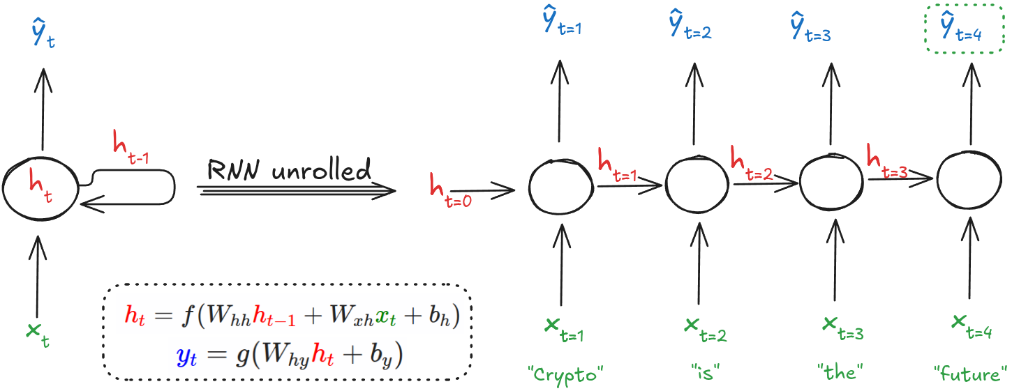Figure 1: RNN Architecture (Image by the author).

The input $\textcolor{green}{x_t}$¶

In a Recurrent Neural Network (RNN), the input at time step $t$, denoted as $\textcolor{green}{x_t}$, represents the data fed into the network at that point in the sequence. It is typically a vector (e.g., a word embedding) in $\mathbb{R}^d$, where $d$ is the embedding dimension.

As an example, lte’s consider the 4-word sentence: $\textcolor{green}{\text{``Cryptocurrency is the future''}}$. This sequence has length $m = 4$. The corresponding inputs are:

Hidden State $\textcolor{red}{h_t}$¶

The hidden state serves as the network’s internal memory, encoding contextual information from the sequence up to time $t$. It is updated as shown above, and plays a key role in maintaining temporal dependencies. At each time step, the hidden state $\textcolor{red}{h_t}$ is updated based on the current input $\textcolor{green}{x_t}$ and the previous hidden state $\textcolor{red}{h_{t-1}}$:

Here $W_{xh}$ and $W_{hh}$ are weight matrices, $b_h$ is a bias vector, and $f$ is a nonlinear activation function such as $\tanh$ or ReLU.

Initial Hidden State $\textcolor{red}{h_0}$¶

The initial hidden state $\textcolor{red}{h_0}$ represents the starting memory of the RNN before any input is processed. It is typically initialized in one of the following ways:

• As a zero vector:
  $\textcolor{red}{h_0} = \mathbf{0} \in \mathbb{R}^n$ where $n$ is the dimensionality of the hidden state.

• With small random values (e.g., sampled from a normal distribution):
  $\textcolor{red}{h_0} \sim \mathcal{N}(0, \sigma^2 I)$

• As a learned parameter:
  $\textcolor{red}{h_0}$ can also be treated as a trainable vector that is learned during training, allowing the model to adapt its initial memory based on the data.

The choice depends on the specific task, model design, and desired behavior at the start of the sequence.

Output $\textcolor{blue}{y_t}$¶

The output at time step $t$ is computed from the hidden state:

where $W_{hy}$ is the output weight matrix, $b_y$ is a bias vector and $g$ is an activation function such as softmax or sigmoid, depending on the task.

RNN Encoder–Decoder¶

The RNN Encoder–Decoder architecture, introduced by Cho et al. (2014) and Sutskever et al. (2014), operates by encoding an input sentence into a fixed-length vector and then decoding it to generate an output sequence.

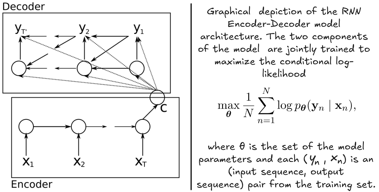
Figure 2: Encode-Decoder architecture (Image and comment from Cho et al. (2014)).

• In this framework, the encoder processes the input sequence ${\textbf{x}} = (\textcolor{green}{x_1}, \textcolor{green}{x_2}, \dots, \textcolor{green}{x_T} )$ and transforms it into a context vector $\textcolor{red}{c}$. Typically, a recurrent neural network (RNN) is employed for this transformation as follows:

and

Here, $\textcolor{red}{h_t} \in \mathbb{R}^n$ represents the hidden state at time step $t$, and the context vector $\textcolor{red}{c}$ is derived from the sequence of hidden states. The functions $f$ and $q$ are nonlinear operations; for example, Sutskever et al. (2014) used an LSTM for $f$ and set $q(\{ \textcolor{red}{h_1}, \dots , \textcolor{red}{h_T} \}) = \textcolor{red}{h_T}$.

• The decoder is trained to generate each word $\textcolor{blue}{y_{t'}}$ based on the context vector $\textcolor{red}{c}$ and the previously generated words $\{\textcolor{blue}{y_1}, \dots , \textcolor{blue}{y_{t'-1}} \}$. It models the probability distribution over the output sequence $\textbf{y}$ by factorizing it into a product of conditional probabilities:

where $\textbf{y} = (\textcolor{blue}{y_1}, \dots , \textcolor{blue}{ y_{T'}} )$.

When using an RNN, each conditional probability is computed as $p(\textcolor{blue}{y_{t'}} | \{\textcolor{blue}{y_1}, \dots , \textcolor{blue}{y_{t'-1}} \}, \textcolor{red}{c}) = g(\textcolor{blue}{y_{t'-1}}, \textcolor{red}{h_{t'}}, \textcolor{red}{c})$, where $g$ is a nonlinear function (possibly multi-layered) that outputs the probability of $\textcolor{blue}{y_{t'}}$, and $\textcolor{red}{h_{t'}}$ denotes the decoder’s hidden state at time $t'$.

Time to Dive into the Implementation 💻¶